Plot flow throughputs with gnuplot in ns3

Topology

N0 (Multiple TCP Senders)---P2Plink(5Mbps,2ms)---N1(Multiple TCP Sinks)

gnuplot-throughput-tcp2.cc (put this file under scratch)

#include <fstream>

#include <string.h>

#include "ns3/core-module.h"

#include "ns3/internet-module.h"

#include "ns3/point-to-point-module.h"

#include "ns3/packet-sink.h"

#include "ns3/packet-sink-helper.h"

#include "ns3/applications-module.h"

#include "ns3/gnuplot.h"

using namespace ns3;

NS_LOG_COMPONENT_DEFINE ("ThroughputTCP2");

const int no=2; /* number of tcp flows */

Ptr<PacketSink> sink[no]; /* Pointer to the packet sink application */

uint64_t lastTotalRx[no]; /* The value of the last total received bytes */

double cur[no];

Gnuplot2dDataset mydata1;

Gnuplot2dDataset mydata2;

void

CalculateThroughput ()

{

Time now = Simulator::Now ();

std::cout << now.GetSeconds ();

for(int j=0;j<no;j++){

cur[j] = (sink[j]->GetTotalRx () - lastTotalRx[j]) * (double) 8 / 1e6;

std::cout << "\t" << cur[j];

lastTotalRx[j] = sink[j]->GetTotalRx ();

// for flow1, the first column is time, the second is throughput

if (j==0) {

mydata1.Add(Simulator::Now ().GetSeconds (), cur[j]);

}

if (j==1) {

mydata2.Add(Simulator::Now ().GetSeconds (), cur[j]);

}

}

std::cout << std::endl;

Simulator::Schedule (MilliSeconds (1000), &CalculateThroughput);

}

int

main (int argc, char *argv[])

{

NS_LOG_INFO ("Create nodes.");

NodeContainer n;

n.Create (2);

InternetStackHelper internet;

internet.Install (n);

NS_LOG_INFO ("Create channels.");

PointToPointHelper pointToPoint;

pointToPoint.SetDeviceAttribute ("DataRate", StringValue ("5Mbps"));

pointToPoint.SetChannelAttribute ("Delay", StringValue ("2ms"));

NetDeviceContainer p2pDevices;

p2pDevices = pointToPoint.Install (n);

Ipv4AddressHelper ipv4;

NS_LOG_INFO ("Assign IP Addresses.");

ipv4.SetBase ("10.1.1.0", "255.255.255.0");

Ipv4InterfaceContainer i = ipv4.Assign (p2pDevices);

NS_LOG_INFO ("Create Applications.");

for(int j=0; j<no; j++) {

PacketSinkHelper sinkHelper ("ns3::TcpSocketFactory", InetSocketAddress (Ipv4Address::GetAny (), 9+j));

ApplicationContainer sinkApp = sinkHelper.Install (n.Get(1));

sinkApp.Start (Seconds (0.0));

sink[j] = StaticCast<PacketSink> (sinkApp.Get (0));

}

ApplicationContainer sourceApps[no];

for(int j=0; j<no; j++) {

BulkSendHelper source ("ns3::TcpSocketFactory", (InetSocketAddress (i.GetAddress (1), 9+j)));

source.SetAttribute ("MaxBytes", UintegerValue (0));

sourceApps[j]=source.Install (n.Get (0));

// To differentiate each applications starting time

double min = 0.0;

double max = 1.0;

Ptr<UniformRandomVariable> x = CreateObject<UniformRandomVariable> ();

x->SetAttribute ("Min", DoubleValue (min));

x->SetAttribute ("Max", DoubleValue (max));

double differ_value = x->GetValue ();

sourceApps[j].Start (Seconds (0.1 + differ_value));

sourceApps[j].Stop (Seconds (20.0));

}

Simulator::Schedule (Seconds (1.0), &CalculateThroughput);

Simulator::Stop (Seconds (22.0));

NS_LOG_INFO ("Run Simulation.");

Simulator::Run ();

Gnuplot plot ("throghput-flow.png");

plot.SetTerminal ("png");

plot.SetLegend ("Time (sec)" , "Throughput (Mbps)");

plot.SetExtra("set yrange [0:5]; set ytics 0,0.5,5");

mydata1.SetTitle("Throughput: flow1");

mydata1.SetStyle(Gnuplot2dDataset::LINES_POINTS);

plot.AddDataset(mydata1);

mydata2.SetTitle("Throughput: flow2");

mydata2.SetStyle(Gnuplot2dDataset::LINES_POINTS);

plot.AddDataset(mydata2);

std::ofstream plotFile ("throghput-flow.plt");

plot.GenerateOutput (plotFile);

plotFile.close ();

Simulator::Destroy ();

NS_LOG_INFO ("Done.");

}

Execution

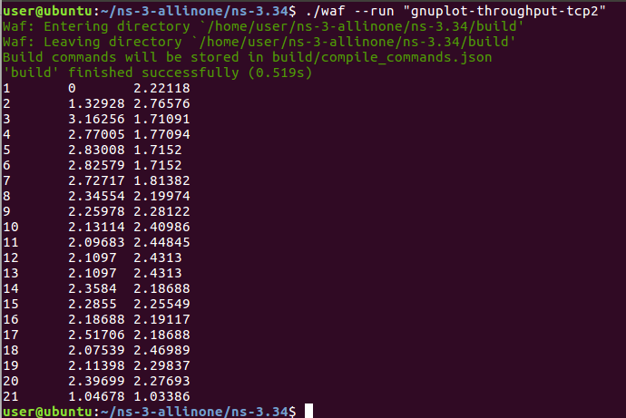
Then you can get throughput-flow.plt.

set terminal png

set output "throghput-flow.png"

set xlabel "Time (sec)"

set ylabel "Throughput (Mbps)"

set yrange [0:5]; set ytics 0,0.5,5

plot "-" title "Throughput: flow1" with linespoints, "-" title "Throughput: flow2" with linespoints

1 0

2 1.32928

3 3.16256

4 2.77005

5 2.83008

6 2.82579

7 2.72717

8 2.34554

9 2.25978

10 2.13114

11 2.09683

12 2.1097

13 2.1097

14 2.3584

15 2.2855

16 2.18688

17 2.51706

18 2.07539

19 2.11398

20 2.39699

21 1.04678

e

1 2.22118

2 2.76576

3 1.71091

4 1.77094

5 1.7152

6 1.7152

7 1.81382

8 2.19974

9 2.28122

10 2.40986

11 2.44845

12 2.4313

13 2.4313

14 2.18688

15 2.25549

16 2.19117

17 2.18688

18 2.46989

19 2.29837

20 2.27693

21 1.03386

e

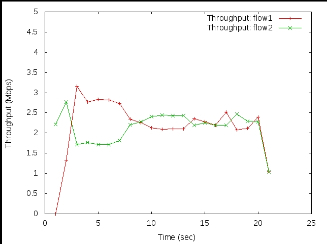
Plot the graph

And then you can get the following figure. (throughput-flow.png)

Back to NS3 Learning Guide

Last Modified: 2022/2/10

Dr. Chih-Heng Ke

Department of Computer Science and Information Engineering, National Quemoy University, Kinmen, Taiwan

Email: smallko@gmail.com